Naive Bayes (NB)

Naive Bayes is a supervised classifier for text classification, and it takes a bag of words view of a document. Word order and grammar are thrown away, so a document is only a set of word counts.

It is called naive because it assumes every word probability is independent of every other word. That assumption is false for real language, and the classifier still works well in practice.

Introduction

For a document $d$ and a class $c$:

$$P(c|d)=\frac{P(d|c)P(c)}{P(d)}$$

where:

• $P(c|d)$ is the probability of $c$ given $d$ is true
• it means what is the probability that the class $c$, given that we are looking at document $d$
• $P(d|c)$ means how well class $c$ explain these words in document $d$
• $P(c)$ represents how common class $c$ is without reading any documents
• $P(d)$ is how liekely is this document overall, across all classes

Step	Rule	Why
1	$c=argma{x}_c(P(c\Vert d))$	the most likely class is the one with the highest probability given document $d$
2	$c=argma{x}_c\left(\frac{P(d\Vert c)P(c)}{P(d)}\right)$	rewrite using Bayes theorem
3	$c=argma{x}_c(P(d\Vert c)P(c))$	drop the denominator
4	$c=argma{x}_c(P(x_1,x_2,x_3\dots x_n\Vert c)P(c))$	a document is its features $x_1\dots x_n$
5	$c=argma{x}_c\left({\prod }_{j}P(x_j\Vert c)P(c)\right)$	the naive assumption, so 1 joint probability becomes a product of separate ones

• $c$ is a variable that stands for a single class label
• $P(d)$ is dropped because it is the same value for every class, so it cannot change which class wins
• step 5 is the only step that is an approximation, and the 4 earlier steps are exact
• argmax returns the class that scores highest, not the score itself

Training

Training is pure counting, and there is no iteration or gradient. Only 2 quantities come out of the training corpus, both by maximum likelihood estimation.

Class prior probability, which is how common the class is:

$$P(c)=\frac{count(docslabelledc)}{count(totaldocs)}$$

Conditional probability, which is how strongly a word points at that class:

$$P(w_i|c)=\frac{count(docswith{w}_{i}labelledc)}{count(docslabelledc)}$$

Zero probability problem

Take a review classifier with classes positive and negative. The word "excellent" appears in review1 but in no other positive review, so:

$$P("excellent"|positive)=0\text{therefore}P(positive|review1)=0$$

• the class score is a product, so a single zero factor drives the whole product to zero
• this as zero probabilities that cannot be conditioned away no matter the evidence, meaning that no amount of other strong evidence can rescue the score
• the trigger is any word unseen for that class in training, which is common because training corpora are finite

Laplace (add-one) smoothing

The fix is to add 1 to every word count, so that no count is ever 0. There are 2 forms:

$$P(w_i|c)=\frac{count(w_i,c)+1}{{\sum }_{w\in V}(count(w,c)+1)}\text{or}P(w_i|c)=\frac{count(w_i,c)+1}{{\sum }_{w\in V}(count(w,c))+|V|}$$

• the 2 forms are the same expression, because adding 1 once for each of the $|V|$ vocabulary terms adds $|V|$ in total
• $V$ is the vocabulary, so $|V|$ is the number of distinct words across the whole corpus and not just the words of 1 class
• the denominator must grow with $|V|$, otherwise the probabilities for a class stop summing to 1

Worked example

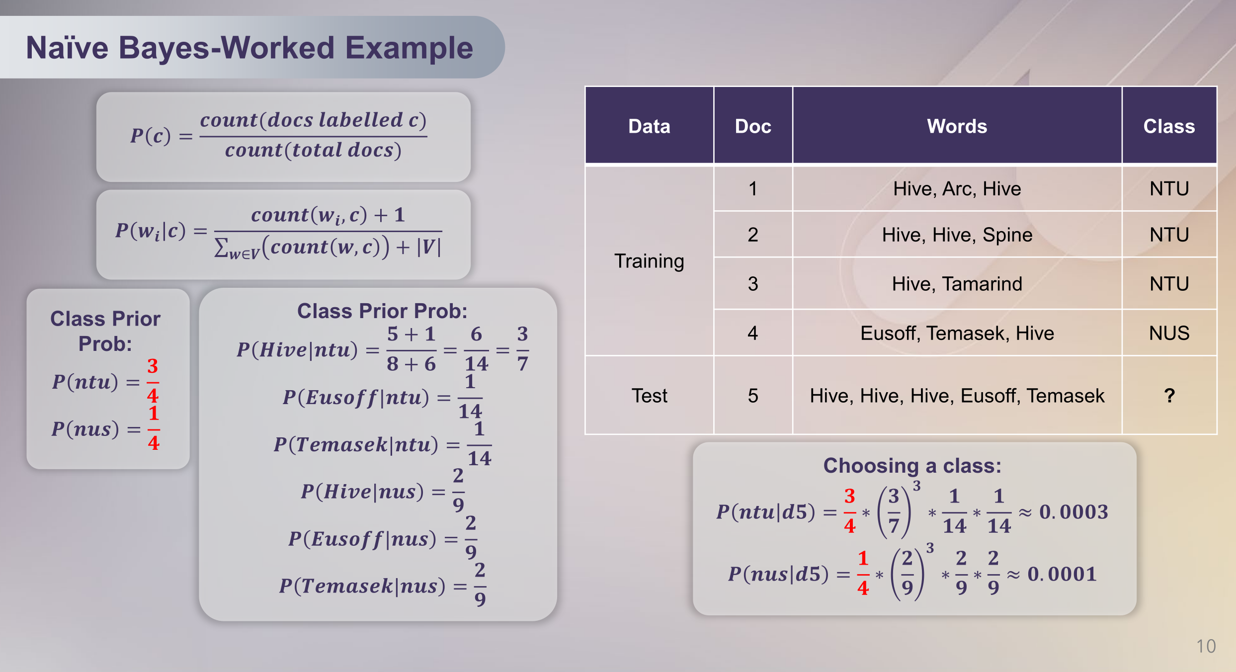
Training data and the test document:

Data	Doc	Words	Class
Training	1	Hive, Arc, Hive	NTU
Training	2	Hive, Hive, Spine	NTU
Training	3	Hive, Tamarind	NTU
Training	4	Eusoff, Temasek, Hive	NUS
Test	5	Hive, Hive, Hive, Eusoff, Temasek	?

The counts behind the numbers:

• vocabulary $V$ = {Hive, Arc, Spine, Tamarind, Eusoff, Temasek}, so $|V|=6$
• NTU holds 8 word tokens in total, of which Hive accounts for 5
• NUS holds 3 word tokens in total, of which each word accounts for 1

Class priors, counted over documents:

$$P(ntu)=\frac{3}{4}P(nus)=\frac{1}{4}$$

Smoothed conditionals, counted over word tokens:

Word	Given NTU	Given NUS
Hive	$\frac{5+1}{8+6}=\frac{6}{14}=\frac{3}{7}$	$\frac{1+1}{3+6}=\frac{2}{9}$
Eusoff	$\frac{0+1}{14}=\frac{1}{14}$	$\frac{2}{9}$
Temasek	$\frac{0+1}{14}=\frac{1}{14}$	$\frac{2}{9}$

Choosing a class for document 5, where Hive appears 3 times so its probability is raised to the power of 3:

$$P(ntu|d5)=\frac{3}{4}\ast {\left(\frac{3}{7}\right)}^3\ast \frac{1}{14}\ast \frac{1}{14}\approx 0.0003$$ $$P(nus|d5)=\frac{1}{4}\ast {\left(\frac{2}{9}\right)}^3\ast \frac{2}{9}\ast \frac{2}{9}\approx 0.0001$$

NTU scores higher, so document 5 is predicted as NTU.

Note

The words unseen in a class still get a non-zero probability, which is $\frac{1}{14}$ here, and that is exactly what smoothing bought. A repeated word contributes its probability once per occurrence, which is why Hive is cubed.

Preprocessing before the classifier

This is the pipeline before fitting the model:

1. use RegEx to strip punctuation and special characters, and lowercase everything
2. apply POS tagging and lemmatise the input words
3. remove stop words
4. apply TF-IDF vectorisation

Code

from sklearn.feature_extraction.text import TfidfVectorizer
from sklearn.model_selection import train_test_split
from sklearn.naive_bayes import MultinomialNB, GaussianNB, CategoricalNB
 
vectorizer = TfidfVectorizer()
X = vectorizer.fit_transform(corpus).toarray()
X_train, X_test, y_train, y_test = train_test_split(X, labels, test_size=0.2)
 
nb = MultinomialNB()
nb.fit(X_train, y_train)
 
predictions = nb.predict(X_test)

Class	Expects	Typical use
MultinomialNB	counts or TF-IDF weights	text classification, and the default choice here
GaussianNB	continuous features	features assumed to follow a normal distribution
CategoricalNB	discrete category codes	features that are labels rather than counts

• fit performs the counting described above, so training is fast
• smoothing is already built in through the alpha parameter, which defaults to 1.0 and gives Laplace add-one
• .toarray() is called because the notebook passes a dense array, although MultinomialNB accepts a sparse matrix as well

Naive Bayes counts words and never draws a boundary, and the model that does draw one is Support Vector Machine (SVM).