Linear Regression

Linear regression learns a linear relationship between input features and a numerical target. It is supervised learning because training examples include their target values.

The equation of the line is modelled as:

$$y=mx+c$$

Loss Function:

$$L(y,t)=\frac{1}{2}(y-t{)}^2$$

To improve this fit, minimise the squared difference between prediction $y$ and target $t$.

Cost Function:

$$J(w,b)=\frac{1}{2N}\sum _{i=1}^N(y^i-t^i{)}^2=\frac{1}{2N}\sum _{i=1}^N(w{x}^i+b-t^i{)}^2$$

Gradient Descent

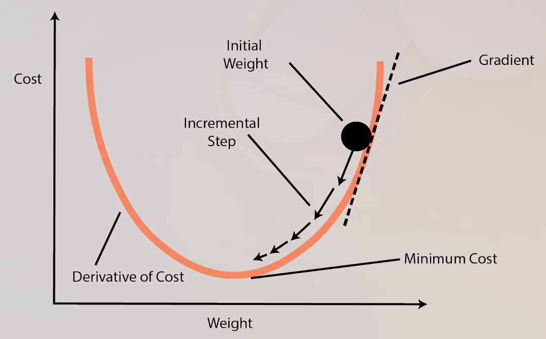
• we apply gradient descent to minimize cost function
• we initialize weights and iteratively adjust them in the direction of steepest descent

At portion of the curve where $\frac{\partial J}{\partial w_j}>0$ (gradient is positive), when we increase $w_j$, $J$ increases.

At portion of the curve where $\frac{\partial J}{\partial w_j}<0$ (gradient is negative), when we increase $w_j$, $J$ decreases.

To decrease the cost function, we can apply:

$$w_j\leftarrow w_j-\alpha \frac{\partial J}{\partial w_j}$$

where $\alpha$ is the learning rate.

Linear regression predicts a continuous value, and the rest of the models used for labels are listed in Text Classification.

---

Code

Fit a numerical relationship

import numpy as np
from sklearn.linear_model import LinearRegression
 
X = np.array([[1.0], [2.0], [3.0], [4.0]])
y = np.array([3.0, 5.0, 7.0, 9.0])
model = LinearRegression()
model.fit(X, y)
predictions = model.predict([[5.0], [6.0]])
print(model.coef_.round(2))         # [2.]
print(round(model.intercept_, 2))   # 1.0
print(predictions.round(2))        # [11. 13.]

Read the data and results:

• X has shape (4, 1): four samples with one feature each
• y has shape (4,): one numerical target per sample
• fit learns a coefficient near 2 and an intercept near 1
• predict accepts two new rows and returns two numerical values
• The learned rule is prediction = 2 * input + 1

LinearRegression fits a least-squares solution. Its fit method performs that calculation internally; this class does not require a manual gradient-descent loop.