Guassian Processes (GP)

A Gaussian Process (GP) is a probabilistic model that defines a distribution over functions. Most models fit 1 best set of tuned/learned parameters and return 1 answer. A GP holds every function that could fit the data, weighted by how plausible each one is, so every prediction arrives with a measure of uncertainty attached.

Instead of modeling data points as fixed parameters, a GP treats entire functions as random variables.

Intuitive Way of thinking of Gaussian Process (GP)

Guassian Process models an unknown function by keeping many possible functions insteaf of choosing only one.

1. Before Seeing Data
GP considers many possible curves. There are infinitely many curves since we can plot an infinite amount of curves to plot 0 points. This is also called prior where we haven't seen the evidence yet.

2. Give the GP Training Data
Now we give the GP a few data points containing input and true output values in the form of (x, y). The training data here is the evidence. The GP gives higher importance to curves that intersect (agree) with all points and lower importance to curves that disagree. The updated collection of possible curves is called posterior.

3. Prediction of $y$ during Training
Given a new input, every curve in the posterior suggests an output. GP will compute the mean and variance of the distribution of these $y_{pred}$ values. The mean is the prediction, while spread is the uncertainty. If its near training data, curves agree closely meaning lower uncertainty, vice versa.

2 Components of a GP

A GP is fully described by 2 functions:

Component	Notation	What it sets
Mean function	$E[f(x_i)]=\mu (x_i)$	the value the function is expected to take before any data is seen
Covariance function	$Cov(f(x_i),f(x_j))=k(x_i,x_j)$	how strongly the values at 2 input points move together

• the covariance function is the same object as a kernel function, so the vocabulary carries over from SVM
• the mean function is often set to 0, which leaves the kernel doing all the work

The kernel Matrix

• $K_x$ is the kernel matrix for the inputs $x$, and its entries are $k(x_i,x_j)$
• this matrix is also known as the gram matrix
• $K_x$ must be positive semidefinite for any $X$, which is the condition that makes it a valid covariance
• this forms a distribution over function values at an arbitrarily finite set of points
• the Kolmogorov Extension Theorem extends that to a distribution over functions, and the result is the Gaussian Process

Prior vs posterior

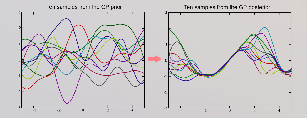
• the width of the spread at any location is the model's uncertainty at that location
• narrow spread means the training data pins the answer down there
• wide spread means the model is guessing, and this is the property that a hard boundary classifier cannot report

The Radial Basis Function (RBF) kernel for GPs

$$K_{RBF}(x_i,x_j)={\sigma }^2\exp \left(-\frac{\Vert x_i-x_j{\Vert }^2}{2l^2}\right)$$

• RBF describes the shape of the function which is a bell shaped bump sitting over a center point
• it creates smooth, infinitely differentiable functions, which suits processes with smooth variations
• $l^2$ is the length scale, and it controls the width of the kernel
• smaller values give more wiggly functions, and larger values give smoother functions
• ${\sigma }^2$ scales the overall size of the variation, so it sets how far the curves swing from the mean

Same RBF kernel as SVM

This is the same RBF kernel used by SVM, written with $l$ in place of $\sigma$ in the denominator. The reading of the width is identical, where a small width means each point influences only its close neighbours.

Code

from sklearn.gaussian_process import GaussianProcessClassifier
from sklearn.gaussian_process.kernels import RBF
 
kernel = 1.0 * RBF(1.0)
clf = GaussianProcessClassifier(kernel=kernel, random_state=0)
 
# Train the model using the training sets
clf.fit(train_review_tfidf, train_sent)
 
# Predict the response for test dataset
y_pred = clf.predict(test_review_tfidf)

• the kernel is built as an object and passed in, rather than named by a string as in svm.SVC(kernel='rbf')
• 1.0 * RBF(1.0) multiplies a constant kernel by an RBF kernel, where the leading 1.0 is ${\sigma }^2$ and the 1.0 inside RBF() is the length scale, $l^2$
• random_state=0 fixes the randomness so the run is reproducible
• clf.predict_proba(X) returns class probabilities, which is the reason to choose a GP over a hard classifier
• this run reports F1 micro of 0.8708, with 158 and 165 errors in the confusion matrix

Comparison with other Regression models

Model	F1 micro on IMDB	What it returns
SVM (RBF)	0.872	a side of a boundary
Gaussian Process	0.8708	a probability with an uncertainty estimate
ELM	0.766	a rounded output value

• the GP score sits level with the SVM score on this dataset, so the uncertainty estimate is what it adds
• the cost is speed, because a GP works with a matrix sized by the number of training documents, which grows badly on large corpora

Kernel functions are shared with Support Vector Machine (SVM), and the RBF kernel appears in both.