Image Filtering

How to Identify the Processing Domain

Domain rule

Spatial-domain processing operates directly on pixel values at positions $(x,y)$. Frequency-domain processing first transforms the image into $F(u,v)$, modifies its frequency components, and transforms it back into an image. The terms low-pass and high-pass describe which frequencies a filter preserves. They do not determine which domain is used to implement the filter.

flowchart TD
    A["Image Enhancement"] --> B["Spatial Domain"]
    A --> C["Frequency Domain"]
    B --> D["Point Processing<br/>One input pixel"]
    B --> E["Spatial Filtering<br/>Pixel neighbourhood"]
    D --> D1["Gray-level reversal, contrast stretching,<br/>clipping, thresholding, log transformation,<br/>histogram equalization"]
    E --> F["Smoothing"]
    E --> G["Sharpening"]
    C --> H["FFT: f(x,y) to F(u,v)"]
    H --> I["Multiply: G(u,v) = H(u,v)F(u,v)"]
    I --> J["IFFT: G(u,v) to g(x,y)"]

Point processing and spatial filtering are both performed in the spatial domain. Point processing uses one corresponding input pixel. Spatial filtering uses a neighbourhood of pixels.

Motivation

• to reduce noise or reduce blur we can't use point processing
• we instead require information about surrounding pixels (neighbourhood)
• therefore we perform something called spatial filtering
• Instead of treating pixels as isolated points, we slide a convolution/filter mask (kernel) over the image grid
• This mask defines a local window (like a 3x3 grid), multiplies the coefficient with the underlying image pixels, and sums them up to write a new value
• this allows us to:
  1. denoise/smooth (using a box or weightage average filter to blend noise away)
  2. sharpen (using a Laplacian or unsharp masking to enhance differences among neighbours)

SPATIAL DOMAIN

This Image Filtering in the Spatial Domain will cover both smoothing and sharpening.

The methods in this section operate directly on $f(x,y)$:

Category	Methods	Operation
Linear smoothing	Box filter, weighted-average filter, spatial Gaussian kernel	Convolution with a neighbourhood kernel
Nonlinear smoothing	Median filter	Sort the neighbourhood and select the median
Derivative filtering	Gradient, Laplacian	Calculate local intensity changes
Sharpening	Composite sharpening, unsharp masking, high-boost filtering	Add or strengthen spatial detail

Key Workflow using Convolution

• slide -> mulitply -> sum -> write
• Normalize by coefficient sum (meaning we have to divide by that sum of pixels in the sliding kernel)
• in otherwords,if our sliding kernel is [1 1 1][1 1 1][1 1 1] then to normalize, we divide by the sum of $1+1+1+1+1+1+1+1+1=9$

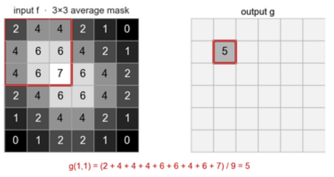
• this image shows the calculation of output $g$ by sliding the kernel

$$g(x,y)=\sum _{s=-a}^a\sum _{t=-b}^{b}w(s,t)f(x+s,y+t)$$

where:

• $f(x,y)$ is the input image
• $g(x,y)$ is the filtered output image
• $w(s,t)$ represents the individual coefficients of the filter mask of size $(2a+1)\times (2b+1)$
• $a$ and $b$ represent the spatial half-width and half-height of the mask
• for example: $a=1$, $b=1$ for a $3\times 3$ neighborhood)

(1) Smoothing

• smoothing/averaging will decrease noise and increase blur
• there is linear and non-linear smoothing

Non-Linear Smoothing (using Median Filter)

The median filter is a spatial-domain neighbourhood filter, but it is not convolution. A median filter takes the median value of pixels in the window and replaces that as the new target value.

Linear Smoothing using Convolution

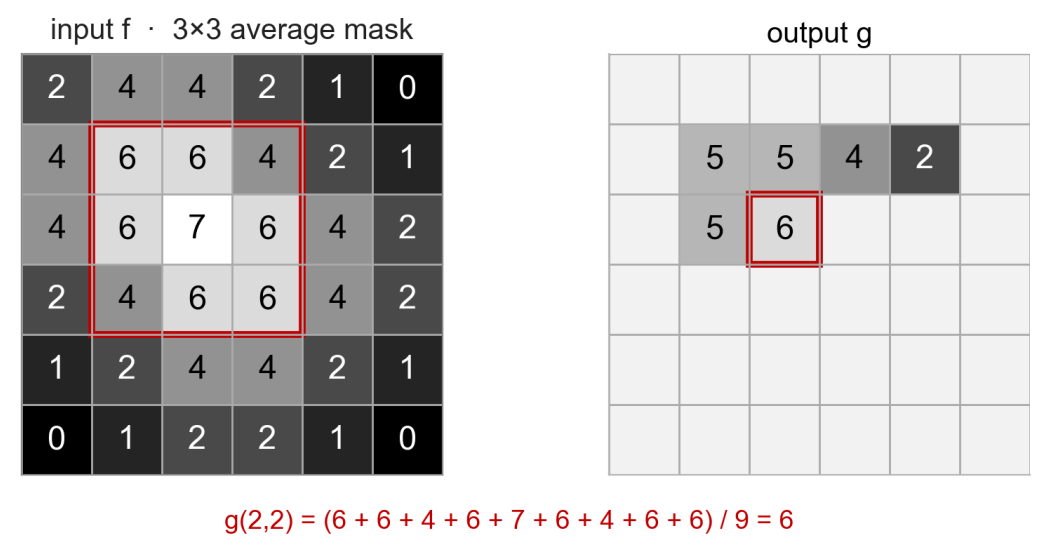
• this image shows how it is calculated, similar to the way we calculate above
• however, the filter/kernel above is just a box (average) filter that is a:

[1 1 1]
[1 1 1]
[1 1 1]

• There are 2 factors that changes the quality of smoothing:
  1. weights in the filter/kernel
  2. size of filter/kernel

1) Weights in the Filter/Kernel

a) Box (Average) Filter

$$\text{Box Filter}=\frac{1}{9}\left[\begin{array}{ccc}1& 1& 1\\ 1& 1& 1\\ 1& 1& 1\end{array}\right]$$

• also called mean or arithmeic mean filter is the simplest smoothing mask
• every pixel in the 3 x 3 neghbourhood is treated with equal importance
• the filter simply sums up the 9 pixels in the window and divides by 9

b) Weighted Average Filter

$$\text{Weighted Average}=\frac{1}{16}\left[\begin{array}{ccc}1& 2& 1\\ 2& 4& 2\\ 1& 2& 1\end{array}\right]$$

• the contains a central bias giving the highest weight of magnitude $4$ to the center pixel
• medium weight of $2$ to the intermediate pixels and lowest weight to the diagonal corner pixels
• This pyramid of weights corresponds to the 2D Gaussian Distrubtion (smooth bell-shaped curve)
• Normalization is performed by dividing matrix by 16 since the sum of of $1+2+1+2+4+2+1+2+1=16$

2. Size of Kernel

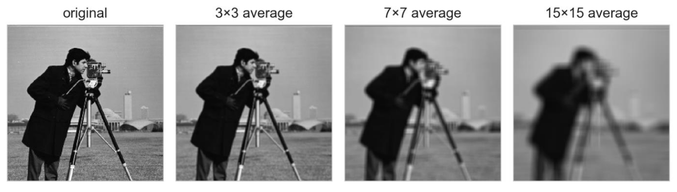
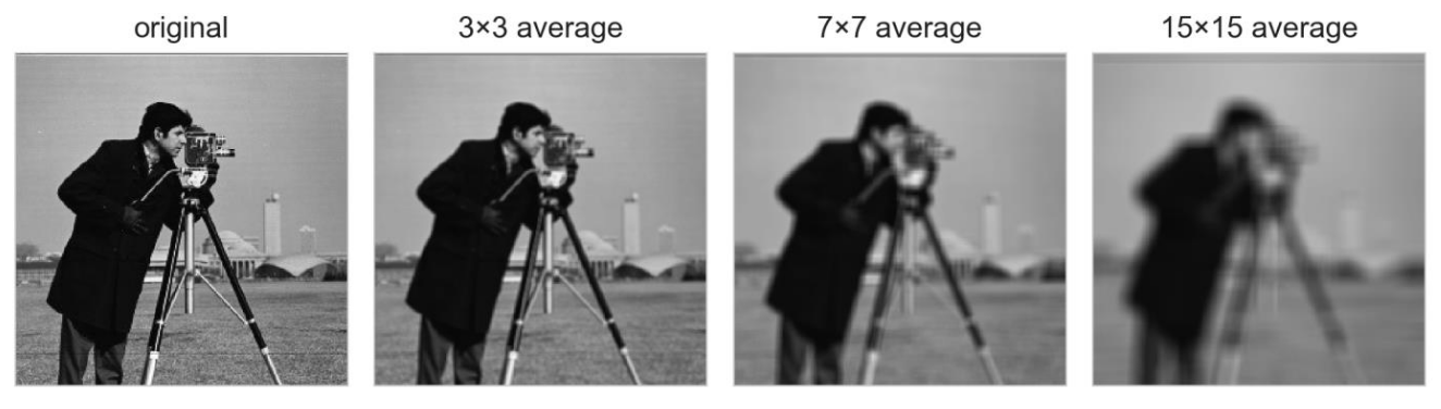
• a larger sized kernel/mask/filter will smooth the image more, thereby bluring the image greatly

(2) Sharpening

• sharpening holds the same meaning as undergoing change
• we therefore use derivatives

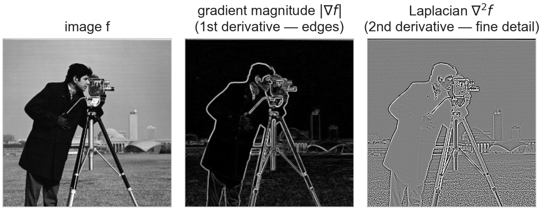
• this image shows what we get when we take the 1st and 2nd derivative of the initial image
• Gradient $|\nabla f|$: detects where the edges are, in otherwords, Edge Detection
• Laplacian ${\nabla }^{2}f$: this shows where the intensity bends, in otherwords Sharpening

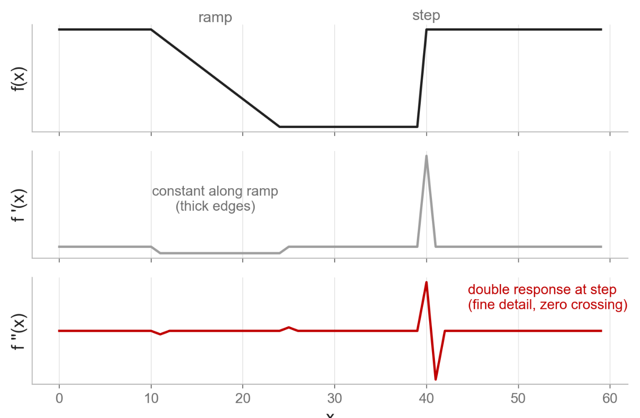
• from the image we can see a comparison of input image with its first derivative and second derivative
• $f$ shows a slow ramp then a sharp step
• $f^{\prime }$ shows a wide bump on the ramp, signifying thick edges
• $f^{\prime \prime }$ shows a $+-$ spike at the step which is finer in detail, where the graph crosses $0$ shows the exact edge in the image

Laplacian

• how we apply this is also by using the kernel/filter
• laplacian is the isotropic (rotation-invariant) second-order derivative operator for 2D images
• 1st derivative (gradient) detects the slope of an edge while the 2nd derivative (Laplacian) detects the "curvature" or where the intensity bends
• There are 2 ways we can achieve a sharpened image:
  1. 2-Step Process using Standard Laplacian Filters (4-neighbour & 8-neighbour)
  2. 1-Step Sharpening Filter

2-Step Process Using Standard Laplacian Filters

First step is to use either the 4-neighbour or the 8-neighbour Laplacian Mask/Kernel/Filter.
4-neighour Laplacian:

$${\nabla }^{2}f=\left[\begin{array}{ccc}0& 1& 0\\ 1& -4& 1\\ 0& 1& 0\end{array}\right]$$

8-neighbour Laplacian:

$${\nabla }^{2}f=\left[\begin{array}{ccc}1& 1& 1\\ 1& -8& 1\\ 1& 1& 1\end{array}\right]$$

• the 8-neighbour laplacian filter is more robust version that includes diagonal neighbours, unlike the 4-neighbour variant

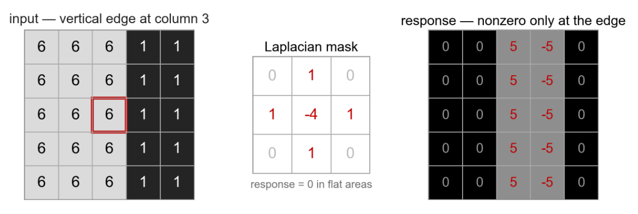
Zero-sum Rule for these 4 and 8 neighbour Laplacian Masks is when we sum all the pixels in the mask, we always get 0. This is a special characteristic of highpass/derivative filters. The characteristic allows us to get 0 on flat areas where all neighbouring pixels have the same intensity.

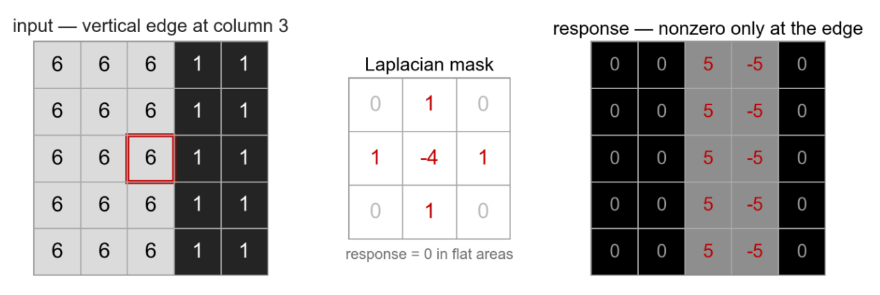
• this image shows the zero sum rule at play
• areas where it is just flat $6$ gets $0$ as the output
• this allows us to get non zero at areas where there are differing values

Second step is to apply the governing formula:

$$g=f-{\nabla }^{2}f$$

• this is subtracting the 2nd derivative of input image from the original input image, pixel to pixel, resulting in out output image, $g$.

2. One-Step Sharpening Filter
This category contains the Composite Sharpening feature which is a single-step function that converts an input image into a sharpened version.

This mask is created by taking an Identity Mask and subtracting the 4-Neighbour Laplacian (we can also use 8-Neighbour Laplacian btw) from it:

$$Identity-Laplacian=Composite$$ $$\left[\begin{array}{ccc}0& 0& 0\\ 0& 1& 0\\ 0& 0& 0\end{array}\right]-\left[\begin{array}{ccc}0& 1& 0\\ 1& -4& 1\\ 0& 1& 0\end{array}\right]=\left[\begin{array}{ccc}0& -1& 0\\ -1& 5& -1\\ 0& -1& 0\end{array}\right]$$

• Sum to One: the sum of all coefficients in this mask is exactly 1 because of subtracting the identity matrix
• Visual Output: convolving with this mask gives a proper normally lit image, where flat regions keep their original brightness and edges are instantly sharpened in a single pass

Unsharp Masking (Introducing the idea only)

• key concept is to sharpen with a blur
• basically we blur the image and then we subtract blur from original image to get a more detailed image
• this is a 3 step pipeline:
  1. Blur original image
  2. Subtract to extract the "detail mask"
  3. Add detail mask back to original image

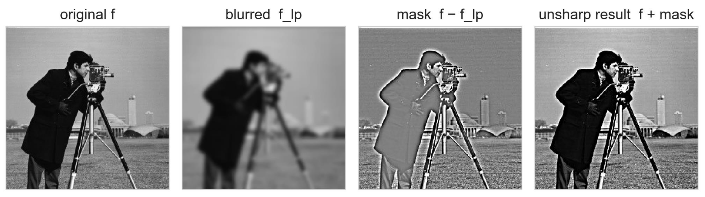
1. Blur original image

• we create a blurred, low-pass filtered copy of the image, $f_{lp}(x,y)$
• this blurred background represents the smooth, low-frequency background information of the scene, with all the sharp edges and details wiped out

2. Subtract to get the "Detail Mask"

$$f_s(x,y)=f(x,y)-f_{lp}(x,y)$$

• $f_s$ is the high-frequency detail map (sharp trasitions, fine lines and edges) or our "Detail Mask" or also called "Unsharp Mask"

3. Add Detail Mask back to Original Image

$$g(x,y)=f(x,y)+A{f}_s(x,y)$$

• this parameter $A$ is the scaling constant that we adjust to control how we sharpen
• $A=1$: unsharp masking (default that yields a clean natural sharpened image)
• $A>1$: called High-Boost Filtering, where we heavily mulitply the detail mask before adding it back. Basically increasing the sharpness

FREQUENCY DOMAIN

Frequency-domain boundary

Everything from this heading through the low-pass and high-pass filter sections uses frequency-domain processing. The input image begins as $f(x,y)$, but the filtering operation is multiplication in $F(u,v)$ rather than neighbourhood convolution on the image pixels.

• an image is just a sum of waves that's why we can look at it in the freq domain

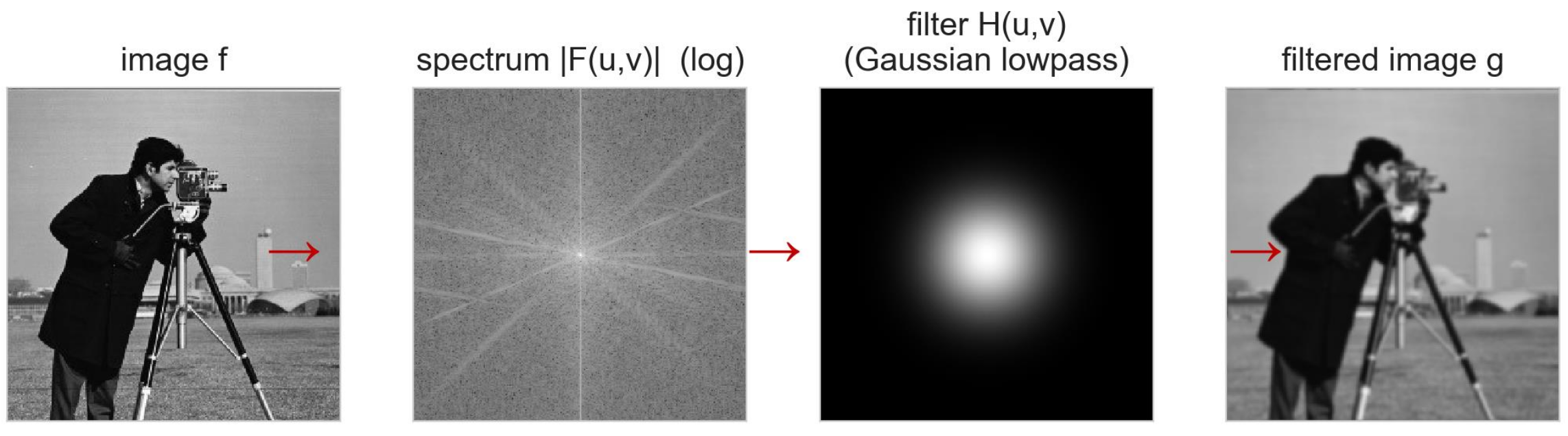
• based on the above image, we can see image $f$ is currently in the spatial domain that consists of high frequency (sharp transitions and fine details) and low frequency content (smooth background regions with very slow, gradual intensity changes)
• we take Fast Fourier Transform (FFT) of our image, which decomposes the picture into a sum of sinusoidal waves of different frequencies and orientations. This gives us a spectrum, $|F(u,v)|$ (log-magnitude)
• the spectrum is centered, meaning the center represents the lowest frequencies (the DC component, which is the average brightness of the image)
• as we move outwards, the frequencies become higher
• the bright "star burst" lines represent the dominant edge directions in the image
• the transfer function of a Guassian Lowpass Filter (GLPF) is used, $H(u,v)$
• in the frequency mask diagram, white (value=1) represents let the frequencies pass through completely
• black (value=0) represents completely block those frequencies
• by converting the filtered spectrum back into the spatial domain, we get the final output, $g$

$$g(x,y)=h(x,y)\ast f(x,y)\iff G(u,v)=H(u,v)F(u,v)$$

• this formula is the governing methodology
• In Spatial Domain, we convolve (apply convolution)
• But in Frequency Domain, we multiply as shown in the equation above

Some properties mentioned above:

• $F(u,v)=\mathrm{FFT}\{f(x,y)\}$
• $g(x,y)=\mathrm{IFFT}\{G(u,v)\}$

Distance Variable

$D(u,v)$ is the distance variable.

$$D(u,v)=[(u-\frac{M}{2}{)}^2+(v-\frac{N}{2}{)}^2{]}^{\frac{1}{2}}$$

• This is the formula for calculating Euclidean Distance from any coordinate point $(u,v)$ in the frequency spectrum to the exact center of the centered Fourier Spectrum $(\frac{M}{2},\frac{N}{2})$ (where M and N are dimensions of the image)
• since lower freqs are nearer to the center, smaller $D$ values represent lower frequencies while a larger $D$ value represents a higher frequency

Ideal Lowpass Filter vs Gaussian Low Pass Filter (for smoothing)

1. Ideal Lowpass Filter (ILPF)

$$H(u,v)=\{\begin{array}{ll}1& \text{if }D(u,v)\le D_0\\ 0& \text{if }D(u,v)>D_0\end{array}$$

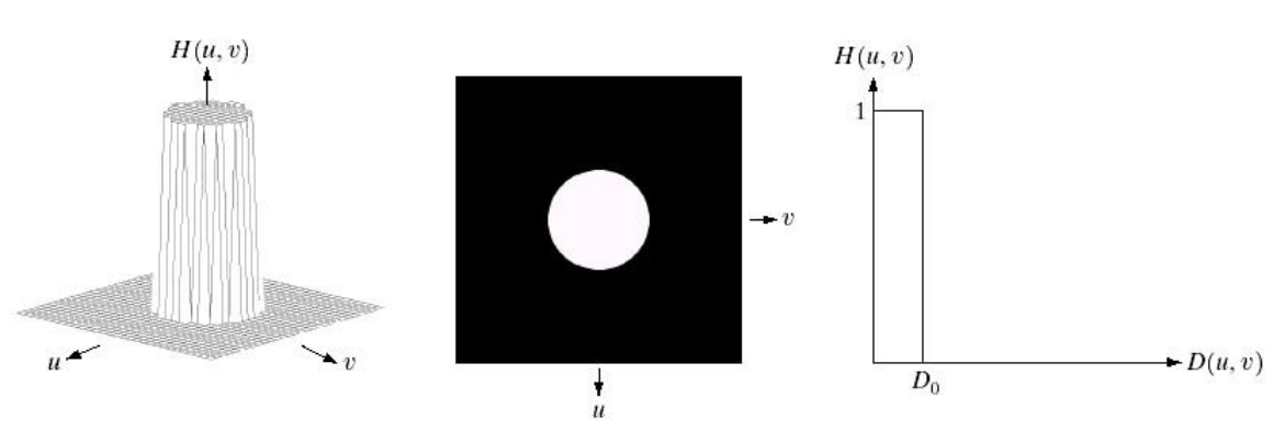
• where: $D_0$ is the user-defined cutoff frequency
• from the image above: we can see 3D view/perspective of this filter where it looks like a a cylinder with vertical walls
• the height is exactly 1
• the filter image (2D view) is a crisp, sharp white circle on a pitch-black background
• this is similar to a mathematical step function
• A disadvantage of lowpass filter is that it will cause ripple effects or echoing around every edge of the image (after we convolve)
  this is because in frequency domain, the lowpass filter is a step function., but in spatial domain, the lowpass filter is a sinc function

2. Guassian LPF: Smooth roll-off

$$H(u,v)=\exp \left(-\frac{D^2(u,v)}{2D_0^2}\right)$$

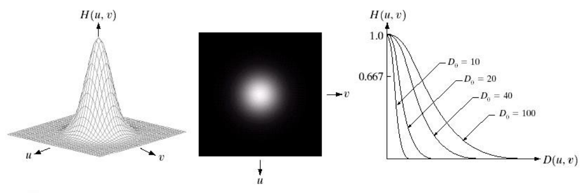
• from the 3D perspective, we can see its a bell shape
• from the 2D perspective, we can also see its blured (grey) and its not a hard cutoff
• we can see how changing $D_0$ affects the steepness (bluriness between 0 and 1) of the curve

0.607 Rule: At $D(u,v)=D_0$, the equation above becomes $H(u,v)=0.607$. This means that the filter's transmission response falls to exactly 60.7% of its maximum value at $D_0$

• the reason why gaussian LPF is preferred over Ideal LPF is because the inverse fourier transform of $H(u,v)$ is also a smooth gaussian curve with no side lobes in the spatial domain
• It therefore doesn't produce any ringing artifacts making it a practical choice for image smoothing

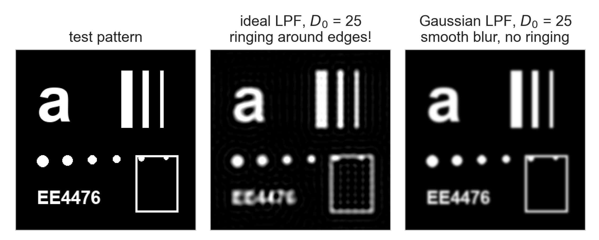
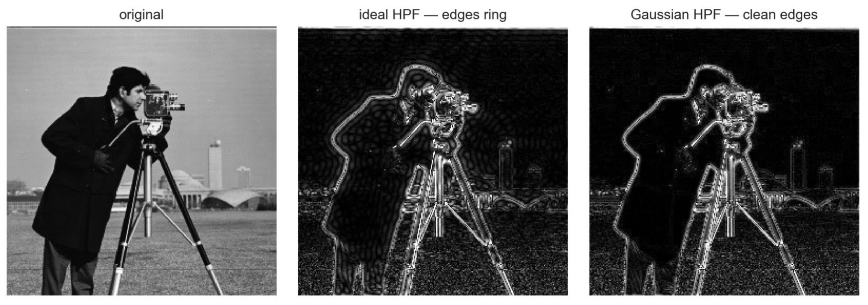
• the above image shows the ringing around edges that is present when using ideal LPF but completely gone when using Guassian LPF

Converting from Low Pass to High Pass

$$H_{hp}(u,v)=1-H_{lp}(u,v)$$

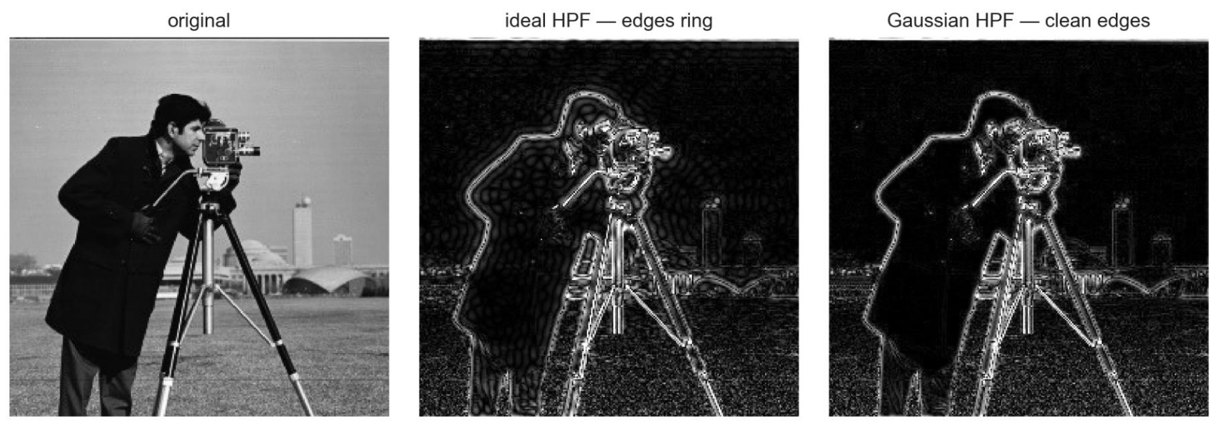
• this formula shows how we can convert low pass to high pass just be subtracting with 1

Same Goal, Different Domain

Goal	Spatial-domain implementation	Frequency-domain implementation
Smoothing	Convolve with a box or Gaussian kernel	Multiply by a low-pass transfer function $H(u,v)$
Sharpening	Use a Laplacian kernel or unsharp masking	Multiply by a high-pass transfer function $H(u,v)$
Remove selected periodic noise	Requires a large or specially designed spatial kernel	Suppress the selected frequencies in the spectrum

Gaussian appears in both domains

A weighted Gaussian matrix is a spatial-domain convolution kernel. A Gaussian low-pass transfer function $H(u,v)$ is a frequency-domain filter. Both produce smoothing, but their calculation steps occur in different domains.

Summary

Goal	Spatial Domain (Masks)	Frequency Domain ($H$)
Smooth/Denoise	Box (Average) Filter, Weighted Average Filter, Median	Lowpass (Gaussian $D_0$)
Sharpen	Laplacian, Unsharp Masking	Highpass ($1-\text{Lowpass}$)

For a small mask/filter like 3x3 or 5x5 averaging mask, we should convolve directly in spatial domain since its computationally cheaper.

If we require precise control such as filtering out specific frequencies (maybe removing periodic diagonal line noise), or if spatial filter is extremely large, its more efficient to use FFT, multiply the arrays and then perform IFFT.