Introduction
Every method in Visual Data Dimensionality Reduction makes features the same way: it picks a direction and measures how far each data point lies along it. This operation is a projection. This note explains it from scratch, and finds the spread of the data along any direction.
Main idea
For a unit vector $\mathbf{u}$, the number $a=\mathbf{u}^T\mathbf{x}$ is the coordinate of $\mathbf{x}$ along $\mathbf{u}$. The point $a\mathbf{u}$ is the closest point on that axis, and the leftover $\mathbf{x}-a\mathbf{u}$ is perpendicular to it. The variance of the data along a unit vector $\boldsymbol{\phi}$ is $\boldsymbol{\phi}^T\boldsymbol{\Sigma}\boldsymbol{\phi}$.
Projecting onto one axis
Take a direction given by a unit vector , which means . The projection of onto this axis gives two things:
How to read them:
- is the coordinate of along the axis, like reading a ruler laid along
- is where lands if you drop it straight down onto the axis
- since , , where is the angle between and
If a direction vector is not of unit length, divide it by its length first, . Otherwise is the coordinate multiplied by .
Example
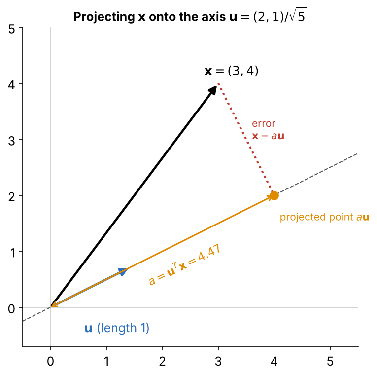
Project onto the direction :
- unit vector:
- coordinate:
- projected point:
- leftover:
The leftover is perpendicular to the axis, since . So , the projected point and the leftover make a right-angled triangle, and Pythagoras holds:
This triangle is the key picture behind principal component analysis.
Coordinate axes
The usual axes are projections too. With :
So the components of a vector are just its coordinates along the standard axes. A projection onto any other unit vector is a coordinate along a new, tilted axis.
Many axes at once
Put unit vectors as the columns of a matrix:
Then one multiplication gives all coordinates:
This is how a -pixel face becomes features: is , and each feature is the coordinate of the face along one learned axis.
Centring first
Usually we project the offset from the mean, , so that a feature measures how far above or below average a sample is along the axis:
Fruit example: an apple with , apple mean , axis :
This axis points toward "wider and taller together", so measures how much bigger than average the apple is.
Variance along a direction
Project every sample onto the unit vector , so . The have mean zero, so their variance is the average of . A number equals its own transpose, so :
Average over the samples, and the middle becomes the covariance matrix:
Apple example with :
| Direction | Meaning | |
|---|---|---|
| , width | 1.0 | spread of width alone |
| , size | the cloud is longest this way | |
| , shape | the cloud is thinnest this way |
The same data spreads by different amounts in different directions. This raises the natural question: which direction has the most spread?
Why do we need this
Projection is the only operation dimensionality reduction uses. Choosing the features means choosing the axes. The formula lets you score any axis by how much of the data's spread it keeps.
Next step
Eigenvectors of a Covariance Matrix finds the directions where is largest and smallest.
Visual 1: centring moves the zero
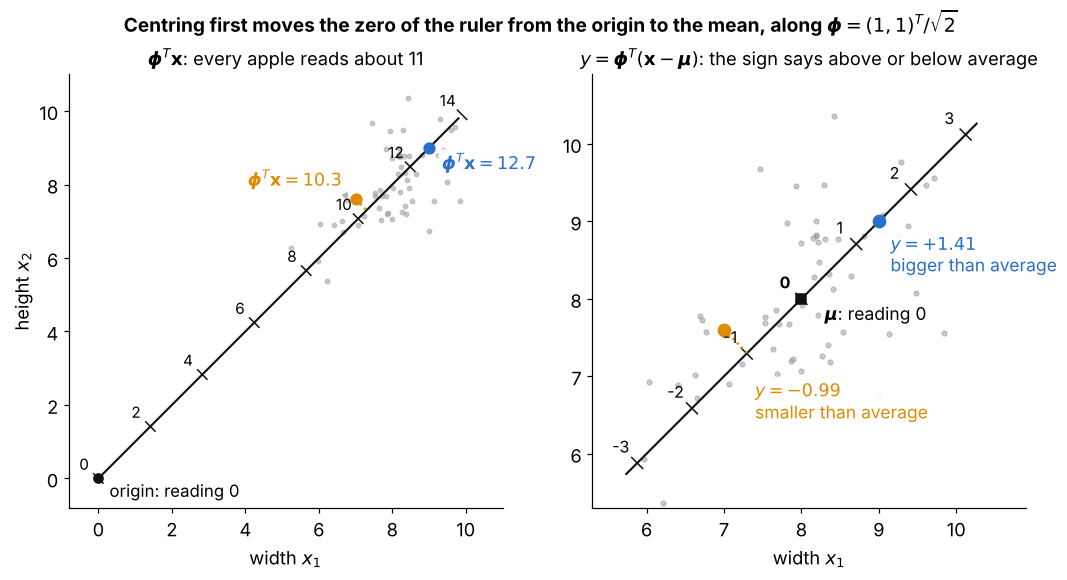
The same apples projected onto , read with two rulers:
- left: measures from the origin, so every apple reads about 11 and the number mostly says how far the cloud is from
- right: puts the zero of the ruler at the mean, so the apple reads , as in the fruit example
- the sign now says above or below average along the axis, and the size says by how much
- the spacing between apples is the same on both rulers, so centring changes only where zero is, not the spread
Visual 2: many axes as one matrix
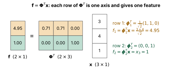
A small case with and , :
- each row of is one unit vector , so the matrix is
- the orange row dotted with gives the orange entry , the coordinate along the tilted axis
- the green row is a standard axis, so the green entry is just the component
- a face uses the same shapes, with of size