Laplacian of Gaussian (LoG)

The Laplacian of Gaussian, or LoG, is an edge-detection filter. It smooths the image, measures a second derivative, and places the edge where the filtered response changes sign.

Main idea

Prewitt and Sobel select large first-derivative responses. LoG selects zero crossings of a smoothed second-derivative response.

---

Why LoG Is Needed

Prewitt and Sobel estimate the first derivative of an image. Their raw edge responses can contain noise and several neighbouring responses around one boundary.

LoG adds Gaussian smoothing before the second derivative is measured:

Stage	Purpose
Gaussian smoothing	Reduce rapid noise changes
Laplacian	Produce positive and negative responses around an intensity transition
Zero-crossing detection	Place the edge where the response changes sign

---

Complete LoG Operation

flowchart LR
    I["Input image"] --> G["Gaussian smoothing<br/>reduce noise"]
    G --> L["Laplacian<br/>second derivative"]
    L --> R["Positive and negative<br/>response lobes"]
    R --> Z["Find the<br/>zero crossing"]
    Z --> E["Edge position"]

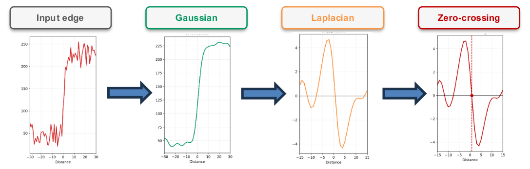
The peaks are not the edge position

The positive and negative peaks show the two sides of the response. The zero crossing between them gives the edge position.

---

Two Equivalent Implementations

LoG can be applied in two ways.

Method 1: Two Filter Passes

1. Convolve the image $f$ with a Gaussian smoothing mask $G$
2. Convolve the smoothed image $f_G$ with the second-derivative mask $L$

$$f_G=f\ast G,g=f_G\ast L$$

Method 2: One Combined LoG Pass

1. Combine the two masks with convolution
2. Convolve the image with the combined mask

$$K_{\mathrm{LoG}}=G\ast L,g=f\ast K_{\mathrm{LoG}}$$

The two discrete forms are equivalent because convolution is associative:

$$\boxed{(f\ast G)\ast L=f\ast (G\ast L)}$$

Here, $\ast$ means two-dimensional convolution. It does not mean ordinary matrix multiplication or element-by-element multiplication.

---

Worked $8\times 8$ Image Example

Consider this $8\times 8$ image:

$$f=\left[\begin{array}{cccccccc}10& 10& 10& 10& 100& 100& 100& 100\\ 10& 10& 10& 10& 100& 100& 100& 100\\ 10& 10& 10& 10& 100& 100& 100& 100\\ 10& 10& 10& 10& 100& 100& 100& 100\\ 10& 10& 10& 10& 100& 100& 100& 100\\ 10& 10& 10& 10& 100& 100& 100& 100\\ 10& 10& 10& 10& 100& 100& 100& 100\\ 10& 10& 10& 10& 100& 100& 100& 100\end{array}\right]$$

The image changes from dark pixels with value $10$ to bright pixels with value $100$. The vertical edge is between columns $4$ and $5$.

Pass 1: Gaussian Smoothing

Use this $3\times 3$ Gaussian mask:

$$G=\frac{1}{16}\left[\begin{array}{ccc}1& 2& 1\\ 2& 4& 2\\ 1& 2& 1\end{array}\right]$$

At an interior position in column $4$, the image neighbourhood is:

$$\left[\begin{array}{ccc}10& 10& 100\\ 10& 10& 100\\ 10& 10& 100\end{array}\right]$$

The smoothed value is:

$$\begin{array}{rl}{f}_G(4)& =\frac{10+20+100+20+40+200+10+20+100}{16}\\ & =32.5\end{array}$$

The corresponding values near the edge become:

Column	Original value	Smoothed value
$3$	$10$	$10$
$4$	$10$	$32.5$
$5$	$100$	$77.5$
$6$	$100$	$100$

The original sharp transition:

$$10,10,100,100$$

becomes the smoother transition:

$$10,32.5,77.5,100$$

Pass 2: Second Derivative

Use this positive-centre second-derivative mask:

$$L=\left[\begin{array}{ccc}0& -1& 0\\ -1& 4& -1\\ 0& -1& 0\end{array}\right]$$

At column $4$, the smoothed neighbourhood is:

$$\left[\begin{array}{ccc}10& 32.5& 77.5\\ 10& 32.5& 77.5\\ 10& 32.5& 77.5\end{array}\right]$$

Therefore:

$$\begin{array}{rl}g(4)& =-32.5-10+4(32.5)-77.5-32.5\\ & =-22.5\end{array}$$

At column $5$:

$$\begin{array}{rl}g(5)& =-77.5-32.5+4(77.5)-100-77.5\\ & =22.5\end{array}$$

Find the Edge

The response changes sign between columns $4$ and $5$:

$$-22.5⟶22.5$$

The zero crossing is therefore between these columns. This is the edge position.

---

Combining the Two Masks

The Gaussian mask and second-derivative mask are combined by two-dimensional convolution:

$$K_{\mathrm{LoG}}=G\ast L$$

For the two $3\times 3$ masks in the worked example:

$$K_{\mathrm{LoG}}=\frac{1}{16}\left[\begin{array}{ccccc}0& -1& -2& -1& 0\\ -1& 0& 2& 0& -1\\ -2& 2& 8& 2& -2\\ -1& 0& 2& 0& -1\\ 0& -1& -2& -1& 0\end{array}\right]$$

Full convolution combines two $3\times 3$ masks into a $5\times 5$ mask:

$$(3+3-1)\times (3+3-1)=5\times 5$$

Applying this combined $5\times 5$ mask once gives the same operation as applying the two $3\times 3$ masks in sequence.

---

How the LoG Equation Creates a Mask

Using the inverted Gaussian convention:

$$h(r)=-\exp \left(-\frac{r^2}{2{\sigma }^2}\right),r^2=x^2+y^2$$

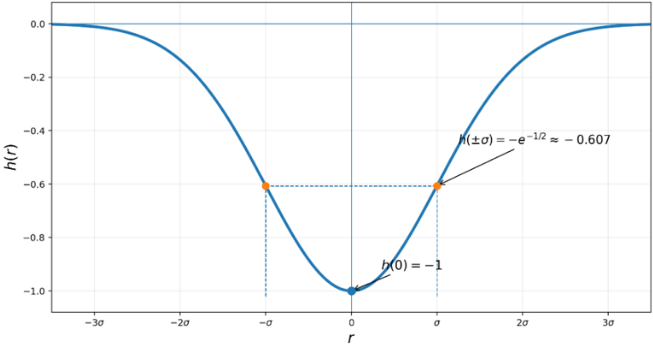
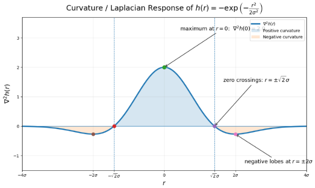
Its two-dimensional Laplacian is:

$${\nabla }^{2}h(r)=\frac{{\partial }^{2}h}{\partial x^2}+\frac{{\partial }^{2}h}{\partial y^2}=-\left(\frac{r^2-2{\sigma }^2}{{\sigma }^4}\right)e^{-r^2/(2{\sigma }^2)}$$

The continuous equation gives the same two implementation choices:

$$\boxed{f\ast {\nabla }^{2}h={\nabla }^2(f\ast h)}$$

Symbol	Meaning
$x,y$	Centred coordinates inside the small filter mask
$r$	Radial distance from the filter centre
$\sigma$	Gaussian scale
$h(r)$	Inverted Gaussian response
${\nabla }^{2}h(r)$	LoG mask coefficient at that position

The symbols $x$ and $y$ are offsets inside the small filter mask. They are not the absolute coordinates of an image pixel.

For a $3\times 3$ mask:

$$x,y\in \{-1,0,1\}$$

For a $5\times 5$ mask:

$$x,y\in \{-2,-1,0,1,2\}$$

For each mask cell:

1. Take its centred coordinates $(x,y)$
2. Calculate $r^2=x^2+y^2$
3. Substitute $r^2$ into the LoG equation
4. Store the result as the coefficient of that mask cell

This process creates the mask once. The same mask then slides across all image positions.

The continuous LoG response has:

• A positive central lobe
• Negative side lobes
• A zero-crossing ring at $r=\sqrt{2}\sigma$
• A negative ring near $r=2\sigma$

Sign convention

The inverted Gaussian gives the LoG a positive centre. Reversing every mask sign exchanges the positive and negative lobes, but the zero-crossing position stays the same. Canny uses a positive Gaussian convention.

---

Effect of $\sigma$

Choice of $\sigma$	Main effect
Smaller $\sigma$	Detects finer changes and retains more noise
Larger $\sigma$	Smooths more strongly and detects structures at a coarser scale

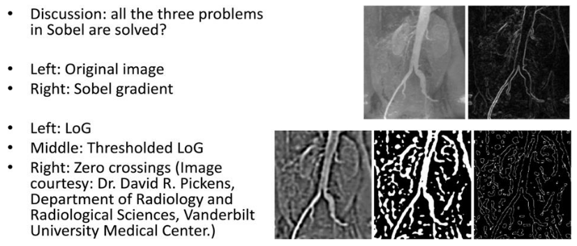
LoG is less sensitive to noise than an unsmoothed second derivative. It still requires a suitable scale and a suitable rule for accepting zero crossings.

---

LoG Compared with Other Edge Detectors

Method	Derivative evidence	Edge decision	Main result
Image Gradient and Edge Detection	First derivative	Large gradient magnitude	Simple candidate edge pixels
LoG	Smoothed second derivative	Zero crossing	Cleaner edge localization
Canny Edge Detector	Smoothed first derivative	Thinned maxima with hysteresis	Thin and connected edge pixels

What to remember

LoG is a filter. Build or select one small LoG mask, slide it across the image, and detect sign changes in the output. The zero crossing, not the response peak, gives the edge position.