Recurrent Neural Networks (RNN)

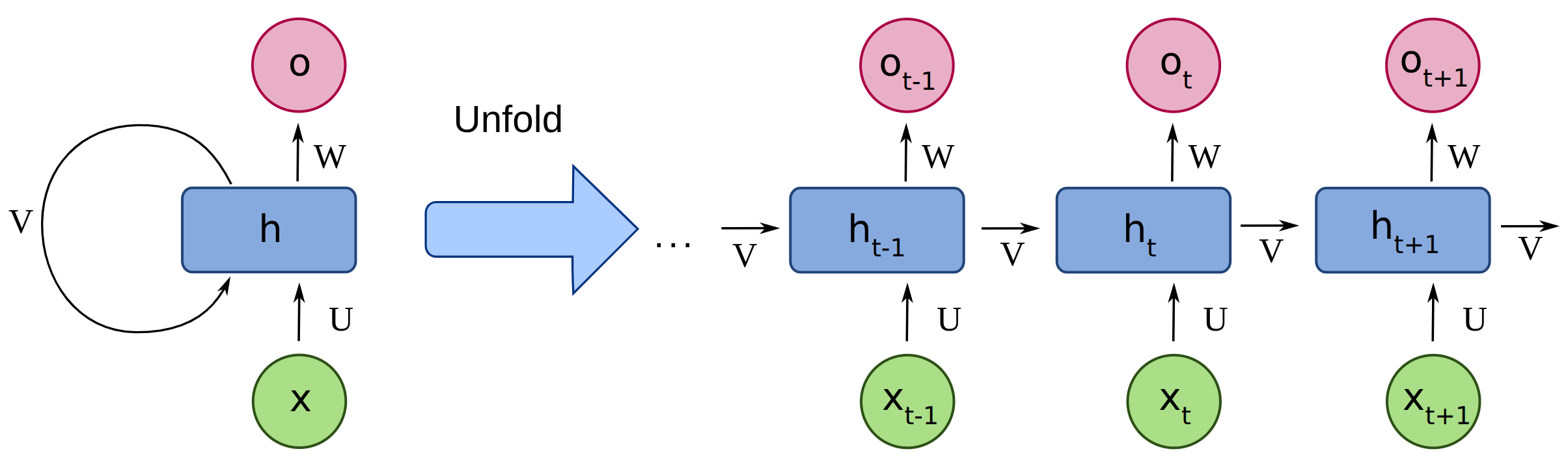
1. Core Concepts

Concept	Explanation
Hidden state ( $h_{t}$ )	The network's "memory" which is updated at each timestep and passed forward
Unrolling	Visualising the RNN as a chain of identical networks, one per timestep
Weight sharing	The same weights $W_{x h}$ , $W_{hh}$ , $W_{h y}$ are reused at every timestep, which enables variable-length sequences From the diagram above, $U$ represents $W_{x h}$ , $V$ represents $W_{hh}$ , $W$ represents $W_{h y}$

2. Main Formulas

The operations inside a standard RNN cell are typically broken down into two steps: updating the memory and calculating the prediction.

An RNN cell computes two things at each timestep:

Hidden state update (memory):

h_{t} = α (W_{x h} x_{t} + W_{hh} h_{t - 1} + b_{h})

Symbol	Meaning
$h_{t}$	New hidden state at timestep $t$
$h_{t - 1}$	Hidden state from the previous timestep
$x_{t}$	Current input at timestep $t$
$W_{x h}$	Weights applied to the input
$W_{hh}$	Weights applied to the previous hidden state
$b_{h}$	Bias term
$α$	Activation function, typically $tanh$ or $R e LU$

Output calculation (prediction):

y_{t} = W_{h y} h_{t} + b_{y}

3. Types of RNNs

Type	Shape	Example use case
Many-to-Many (Synced)	Input at every step, output at every step	Stock price forecasting, video frame classification
Many-to-One	Full sequence in, single output	Sentiment analysis, spam detection
One-to-Many	Single input, sequence output	Image captioning
Many-to-Many (Delayed)	Encoder compresses sequence and then Decoder generates sequence	Machine translation

Choosing the model and output

A simple RNN can be useful for short sequences or as a small baseline. Compare validation results with LSTM or GRU when the task needs information from distant positions.

Choose the output to match the target:

One label per sequence: use a representation of the complete sequence
One label per token: keep the hidden state at every position

Sigmoid produces values between zero and one, which makes it useful for gates and binary probabilities. Tanh produces values between minus one and one, which makes it useful for hidden states. Both can have small derivatives when their inputs are far from zero.

4. Backpropagation Through Time (BPTT)

Training an RNN requires a time-aware variant of backpropagation called BPTT

Process

Forward pass --> compute outputs from $t = 1$ to $t = T$
Calculate loss --> evaluate prediction error at relevant timesteps
Backward pass --> compute gradients from $t = T$ back to $t = 1$
Sum gradients --> because weights are shared, the total gradient for $W_{x h}$ is the sum of its gradients across all timesteps
Weight update --> apply SGD / Adam to minimise loss

Vanishing & Exploding Gradients

BPTT repeatedly combines recurrent weights and activation derivatives as it sends gradients through time.

Problem	Cause	Effect
Vanishing gradients	Repeated products become very small	Earlier positions receive weak learning signals
Exploding gradients	Repeated products become very large	Training can become unstable

LSTM and GRU gates help preserve useful learning signals. Gradient clipping limits large gradients.

5. Why the problems arise

Vanishing Gradient's Cause

Treating a single RNN cell as a function $f$ , the hidden state nests recursively:

Timestep	Hidden state
$t = 1$	$h_{1} = f (x_{1}, h_{0})$
$t = 2$	$h_{2} = f (x_{2}, f (x_{1}, h_{0}))$
$t = 3$	$h_{3} = f (x_{3}, f (x_{2}, f (x_{1}, h_{0})))$

By timestep 3, the hidden state depends on three recurrent calculations. During backpropagation, repeated multiplication by small derivatives can weaken the learning signal sent to early positions.

Exploding Gradient's Cause

For a tanh RNN:

Tanh bounds the forward hidden-state values between minus one and one
Backpropagation uses derivatives of tanh and the recurrent weights
Their repeated products can grow large, even when the forward hidden states are bounded

Code

PyTorch: follow one batch

import torch
from torch import nn
 
class RNNModel(nn.Module):
    def __init__(self, vocab_size, embedding_dim, hidden_dim, output_size):
        super().__init__()
        self.embedding = nn.Embedding(vocab_size, embedding_dim)
        self.rnn = nn.RNN(embedding_dim, hidden_dim, batch_first=True)
        self.fc = nn.Linear(hidden_dim, output_size)
# batch_first=True means we input into hidden state row by row
# if not it will be index (1,1) then (1,2) etc
 
    def forward(self, x):
        embedded = self.embedding(x)
        output, hidden = self.rnn(embedded)
        return self.fc(output)
 
x = torch.tensor([[1, 2, 3, 4], [2, 3, 4, 5]], dtype=torch.long)
model = RNNModel(10, 8, 16, 10)
logits = model(x)
print(tuple(logits.shape))  # (2, 4, 10)

Read the model definition:

nn.Module is the base class for a PyTorch model
__init__ creates the layers once; super().__init__() initialises the base class
Layers assigned to self become registered parts of the model
model(x) calls forward, which defines the path through those layers
batch_first=True gives the order (batch, sequence, features)
self.fc(output) applies the same prediction layer to every token position

Follow the shapes:

Value	Shape	Meaning
`x`	`(2, 4)`	Two sequences of four token IDs
`embedded`	`(2, 4, 8)`	Vector Embedding of 8 dims per token
`output`	`(2, 4, 16)`	Combined output from hidden states at each position
`hidden`	`(1, 2, 16)`	Final state of the single recurrent layer / Final Output from the final hidden state
`logits`	`(2, 4, 10)`	Ten raw scores per position

Note the hidden value above. We know that the output from all hidden layers have the same shape of (2, 1, 16) meaning this shape is also the output from the last hidden state. However, PyTorch's hidden format leaves out the position dimension, because hidden always contain the final position.

Our idea is (2, 1, 16) which is sentence x position x values but instead, we represent it as (1, 2, 16) which is layers_of_rnn x sentences x values.

For one prediction per sequence, change the final line to return self.fc(hidden[-1]). The output then has shape (2, 10). For this single-direction model, output[:, -1, :] also selects the final state when every sequence fills all four positions.

The model starts with random weights. See Pretraining Loop for the training steps. PyTorch RNN reference.

TensorFlow/Keras: Training of RNN to classify complete reviews

import tensorflow as tf
 
reviews = tf.constant([
		"good film",
		"bad film",
		"good story",
		"bad story"
])
 
labels = tf.constant([[1.0], [0.0], [1.0], [0.0]])
encoder = tf.keras.layers.TextVectorization(
    max_tokens=1000, output_mode="int", output_sequence_length=4)
# this is used to convert text into sequences of word IDs
 
encoder.adapt(reviews)
# adapt learns the vocabulary from the training reviews
 
model = tf.keras.Sequential([
    tf.keras.Input(shape=(), dtype=tf.string),
    encoder,
    tf.keras.layers.Embedding(len(encoder.get_vocabulary()), 8, mask_zero=True),
    tf.keras.layers.SimpleRNN(16),
    tf.keras.layers.Dense(1),
])
model.compile(
    optimizer=tf.keras.optimizers.Adam(learning_rate=0.001),
    loss=tf.keras.losses.BinaryCrossentropy(from_logits=True),
    metrics=[tf.keras.metrics.BinaryAccuracy(threshold=0.0)],
)
history = model.fit(reviews, labels, batch_size=2, epochs=2, verbose=0)
logits = model(reviews, training=False)
print(tuple(logits.shape))  # (4, 1)

Read the operations:

max_tokens=1000: Allow up to 1,000 vocabulary entries, including reserved entries
output_mode="int": Represent each word with an integer ID
output_sequence_length=4: Give each review four positions, adding padding or removing extra words
adapt learns the vocabulary from the training reviews
output_sequence_length=4 pads or truncates each sequence to four IDs
mask_zero=True tells compatible later layers to ignore padding positions
SimpleRNN(16) returns one 16-value state per review by default
Dense(1) produces one binary logit per review
compile selects the loss and optimiser; fit performs the training updates
Logits use a decision threshold of zero; sigmoid probabilities use 0.5

Sequential connects the layers in order:

Review text
    ↓ encoder
Word IDs
    ↓ Embedding
Word vectors
    ↓ SimpleRNN
Final hidden state for each review
    ↓ Dense
One prediction score for each review

This is a small example of the code path. Use separate validation and test data when measuring performance. Keras text encoder reference.

JJ

Explorer