Gated Recurrent Units (GRU)

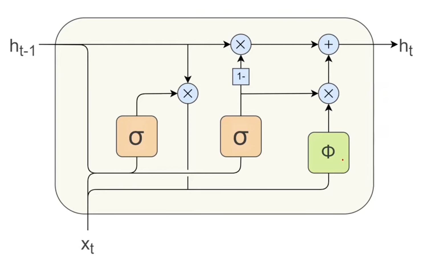
A GRU is a streamlined version of the LSTM that achieves similar performance with fewer gates and less computation. It merges the LSTM's cell state and hidden state into a single hidden state $h_t$, and uses only two gates to control information flow.

---

Overview

Property	GRU	LSTM
Gates	2 (Reset + Update)	3 (Forget + Input + Output)
Internal networks	3	4
Memory mechanism	Single hidden state $h_t$	Separate cell state + hidden state
Long-term memory	Depends on the task and training	Depends on the task and training
Computation	Lower	Higher

---

Gate 1: Reset Gate

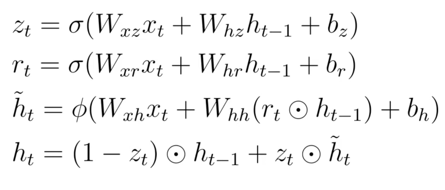
The Reset Gate $r_t$ controls how much of the previous hidden state is allowed to influence the candidate hidden state, similar to the Forget Gate in an LSTM.

Formula:

$$r_t=\sigma (W_{xr}{x}_t+W_{hr}{h}_{t-1}+b_r)$$

1. Take the previous hidden state $h_{t-1}$ and current input $x_t$
2. Multiply by their respective weight matrices $W_{xr}$, $W_{hr}$ and add bias $b_r$
3. Apply sigmoid --> output $r_t\in (0,1)$
4. $r_t$ is multiplied element-wise with $h_{t-1}$ before feeding into the candidate state

A value near 0 means "forget most of the past"; near 1 means "keep most of the past".

---

Candidate Hidden State

The Candidate Hidden State, $\widetilde{h_t}$, is a proposed new hidden state which is similar to what we could set $h_t$ to:

$${\tilde{h}}_t=\tanh (W_{xh}{x}_t+W_{hh}(r_t\odot h_{t-1})+b_h)$$

1. Current input $x_t$ is projected by $W_{xh}$
2. Previous hidden state $h_{t-1}$, gated by $r_t$ (element-wise), is projected by $W_{hh}$
3. Sum both projections, add bias $b_h$, apply tanh --> output in $(-1,1)$

The reset gate determines how much of $h_{t-1}$ shapes this candidate.

---

Gate 2: Update Gate $z_t$ --> Final Hidden State $h_t$

The Update Gate decides how much of the candidate to accept vs. how much of the old hidden state to carry forward:

$$z_t=\sigma (W_{xz}{x}_t+W_{hz}{h}_{t-1}+b_z)$$ $$h_t=z_t\odot {\tilde{h}}_t+(1-z_t)\odot h_{t-1}$$

• $z_t\approx 1$: take mostly from the candidate (new information wins)
• $z_t\approx 0$: keep mostly the old hidden state (memory is preserved)

The final $h_t$ is a weighted blend of the old memory and the new candidate, controlled entirely by $z_t$.

---

Gate conventions in implementations

The equation above uses $z_t$ as the fraction of the candidate to accept. PyTorch uses $z_t$ as the fraction of the old state to retain. Under that convention, a gate near one keeps old information.

PyTorch also applies the reset gate after the previous state has been linearly transformed when calculating the candidate. The earlier formula applies the reset gate before that transformation. Read the implementation's equation when matching its internal values. PyTorch GRU reference.

GRU vs. LSTM

	LSTM	GRU
Gates	Forget, Input, Output	Reset, Update
Internal networks	4	3
Long-term memory	Separate cell state can help	Gated hidden state can retain context
Computation cost	Higher	Lower
When to use	Test when a separate cell state helps	Test when a smaller recurrent cell is useful

---

Code

PyTorch

import torch
from torch import nn
 
ids = torch.tensor([[1, 2, 3], [3, 2, 1]], dtype=torch.long)
embedding = nn.Embedding(10, 8)
gru = nn.GRU(8, 16, batch_first=True)
head = nn.Linear(16, 2)
output, h_n = gru(embedding(ids))
logits = head(h_n[-1])
print(tuple(output.shape))  # (2, 3, 16)
print(tuple(h_n.shape))     # (1, 2, 16)
print(tuple(logits.shape))  # (2, 2)

Read the data path:

• embedding(ids) has shape (2, 3, 8)
• nn.GRU(8, 16) accepts eight features and stores sixteen hidden values per position
• output contains all positions; h_n contains the final state
• The GRU returns one state tensor; LSTM returns hidden and cell state tensors
• head(h_n[-1]) produces two scores for each complete sequence

For one prediction per token, use head(output) to obtain (2, 3, 2).

Bidirectional GRU Shape Example

x = torch.zeros(3, 4, 8)
gru = nn.GRU(
    input_size=8,
    hidden_size=5,
    bidirectional=True,
    batch_first=True,
)
output, hidden = gru(x)
 
summary = torch.cat((hidden[0], hidden[1]), dim=1)
head = nn.Linear(10, 2)
scores = head(summary)
 
print(tuple(output.shape))   # (3, 4, 10)
print(tuple(hidden.shape))   # (2, 3, 5)
print(tuple(summary.shape))  # (3, 10)
print(tuple(scores.shape))   # (3, 2)

Read the input and layer arguments:

• x has three sequences, four time steps, and eight input features per time step
• input_size=8 matches the eight values in each $x_t$
• hidden_size=5 gives each direction a five-dimensional hidden state
• bidirectional=True creates a forward direction and a backward direction

Read the returned tensors:

Tensor	Shape	Meaning
output	(3, 4, 10)	Both directions at every time step from the final GRU layer
hidden	(2, 3, 5)	Final state of each direction
hidden[0]	(3, 5)	Final forward state
hidden[1]	(3, 5)	Final backward state

PyTorch concatenates the two direction sizes in output, so 5 + 5 gives the final size 10. A separate-direction view would have shape (3, 4, 2, 5), but PyTorch returns (3, 4, 10).

batch_first=True changes the input and output order. It does not change the hidden order, which remains (layers * directions, batch, hidden size).

For one sequence-level prediction, torch.cat(..., dim=1) joins the five forward values and five backward values for each batch item:

(3, 5) + (3, 5) -> (3, 10)

TensorFlow/Keras

import tensorflow as tf
 
ids = tf.constant([[1, 2, 3], [3, 2, 1]])
embedded = tf.keras.layers.Embedding(10, 8)(ids)
gru = tf.keras.layers.GRU(16, return_sequences=True, return_state=True)
output, h_n = gru(embedded)
logits = tf.keras.layers.Dense(2)(h_n)
print(tuple(output.shape))  # (2, 3, 16)
print(tuple(h_n.shape))     # (2, 16)

return_state=True adds the final hidden state to the output. return_sequences=True keeps all token positions in output. In a Sequential classifier, replacing LSTM(16) with GRU(16) uses the GRU's final state by default.

Stacked GRU Shape Example

model = tf.keras.Sequential([
    tf.keras.Input(shape=(5, 8)),
    tf.keras.layers.GRU(6, return_sequences=True),
    tf.keras.layers.GRU(4),
    tf.keras.layers.Dense(2),
])

Keras interprets Input(shape=(5, 8)) as five time steps and eight input features for one sample. The runtime input includes the batch dimension and has shape (batch, 5, 8).

At time step t, the first GRU receives the row inputs[:, t, :] with shape (batch, 8). It combines this row with the previous hidden state and produces a new hidden state with six dimensions.

With five time steps, the first GRU calculates five hidden states:

x_1 + h_0 -> h_1
x_2 + h_1 -> h_2
x_3 + h_2 -> h_3
x_4 + h_3 -> h_4
x_5 + h_4 -> h_5

GRU(6) means six hidden units, so each hidden-state vector has six dimensions. It does not mean six time steps or six separate hidden states.

The shape path is:

(batch, 5, 8)
      -> GRU(6, return_sequences=True)
(batch, 5, 6)
      -> GRU(4)
(batch, 4)
      -> Dense(2)
(batch, 2)

return_sequences=True returns all five hidden states from the first GRU. The second GRU needs this three-dimensional sequence input. Without return_sequences=True, the first GRU would return only h_5 with shape (batch, 6).

The second GRU returns its final four-dimensional hidden state. Dense(2) then uses all four values to produce two output scores.